We used the underactuated cartpole system to compare model-based planning and model-free learning under a common stabilization task. Dynamic programming solves a discretized model globally, MPC repeatedly optimizes a continuous finite-horizon trajectory, iLQR supplies local feedback around a nominal trajectory, and Q-learning estimates action values directly from sampled interaction.
Our study follows the complete control pipeline: how the objective shapes a value function, how planning horizon affects closed-loop control, how learning schedules influence a tabular agent, and how the methods trade performance against computation and adaptability. The separate breathing sine-wave trajectory-tracking study is presented on the Cartpole MPC project page.
With only a terminal penalty, the value function approximately measures discounted time to failure. Increasing the discount factor spreads the high-cost boundary inward because future failures matter more. Adding a dense quadratic cost creates smoother gradients, although excessively large weights discourage the cart motion needed to stabilize the pole.
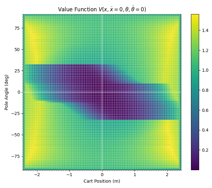
Increasing the state-grid resolution sharpened the estimated recovery boundary. At the highest feasible resolutions, the zero-velocity slice suggested recovery from approximately $32^\circ\pm1^\circ$. This interpretability comes with a steep cost: a four-dimensional grid grows as $R^4$, and memory limited our experiments beyond $R=90$.
Figure 1. High-resolution DP value-function slice showing the estimated recoverable region for zero cart and angular velocity.
Short-horizon MPC is too short-sighted to build the cart motion needed for later recovery. Across 100 evaluation episodes, the first horizon with no terminations was $H=9$. A stricter performance target required more foresight: the mean return first fell below $0.01$ at $H=30$.
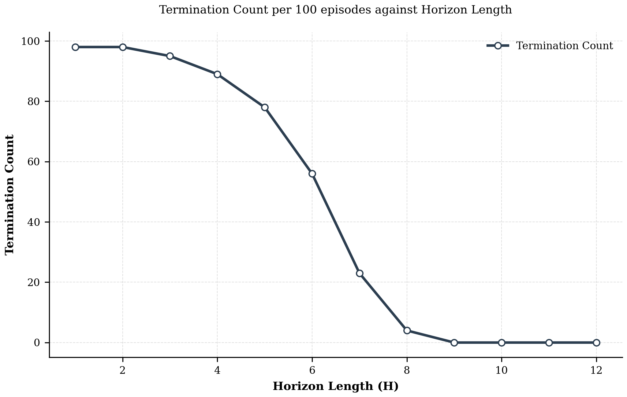
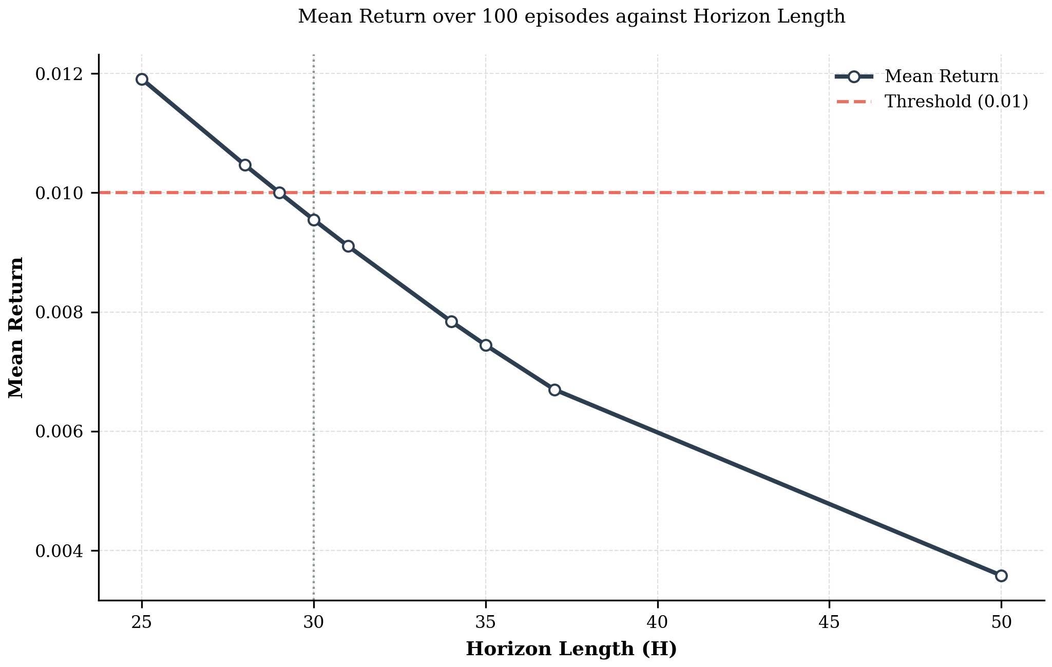
Figure 2. Episode terminations and mean return as the MPC planning horizon increases.
In our implementation, MPC maintained a 100% survival rate through disturbance level 5, whereas iLQR remained perfect through level 155. This result reflects the specific setup rather than a universal advantage: iLQR used a full-episode horizon and immediately applied its local feedback gains, while MPC used a shorter horizon and responded through re-optimization at the following timestep.
For a caregiving robot, we would still prefer MPC as the starting point. It re-plans from the latest measured human state and can explicitly incorporate safety constraints and uncertainty. Standard iLQR remains local to a nominal trajectory and requires additional constraint handling for unpredictable human motion.
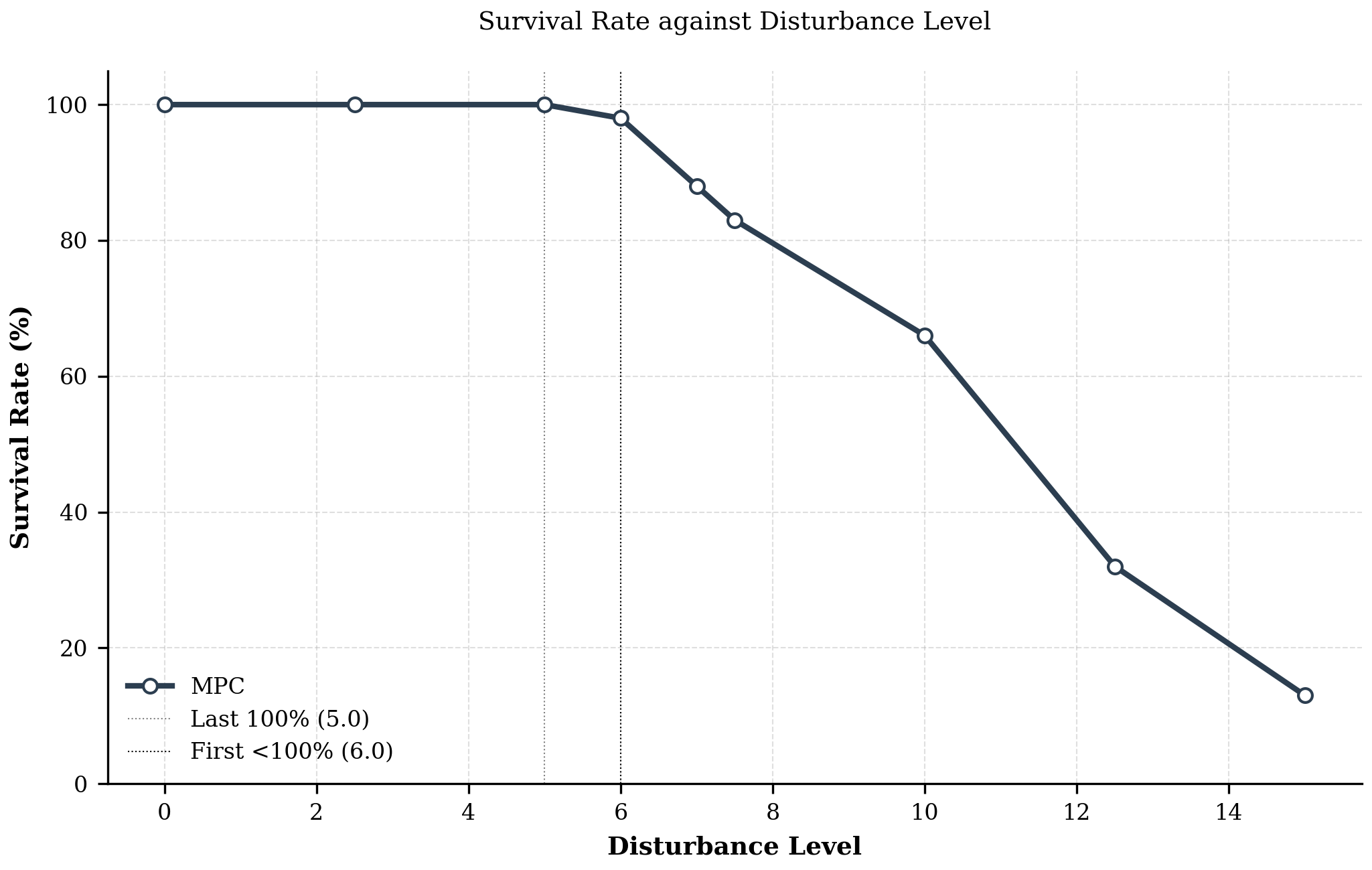
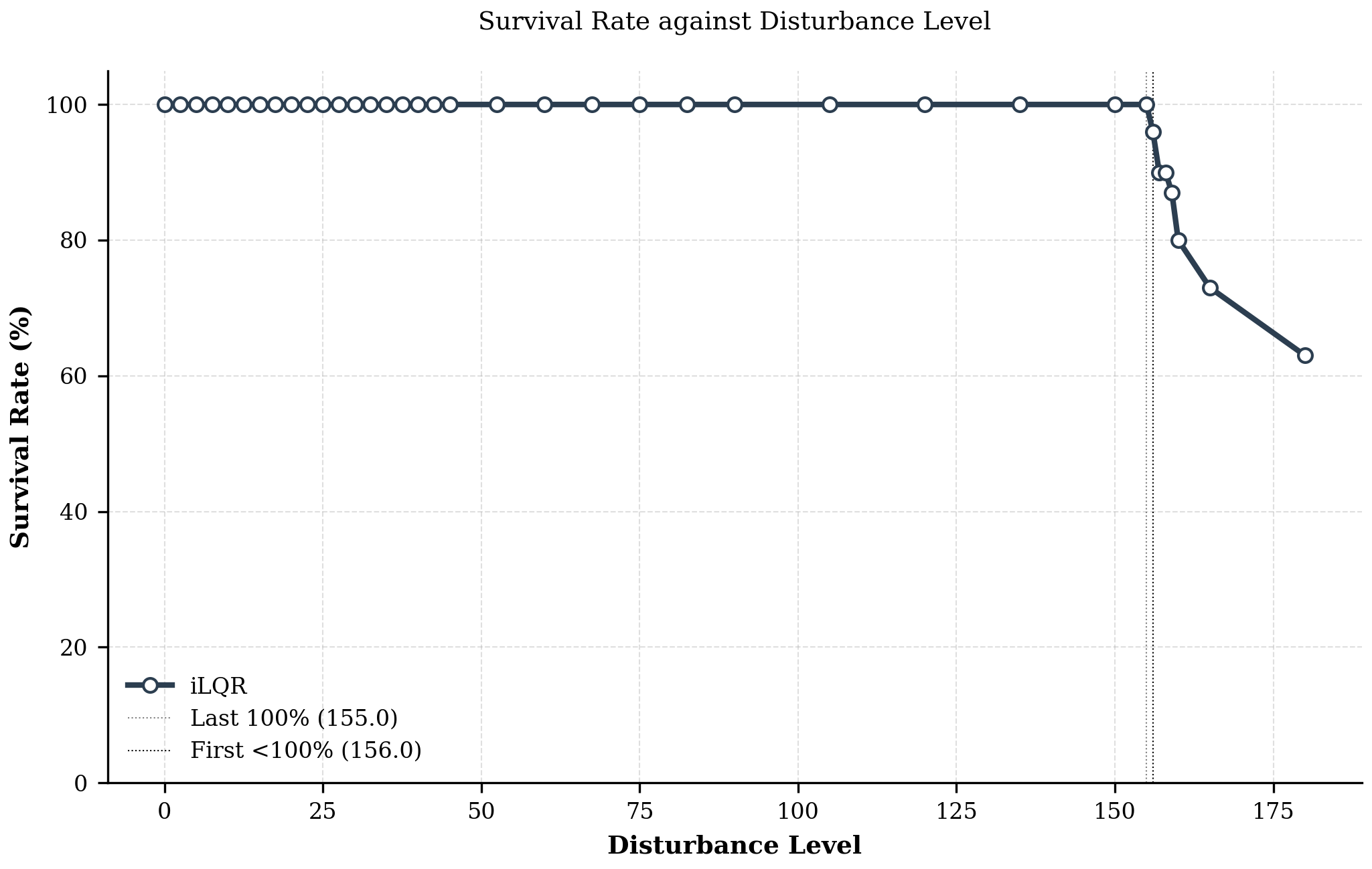
Figure 3. Survival rate under increasing disturbances for MPC and iLQR in our experimental setup.
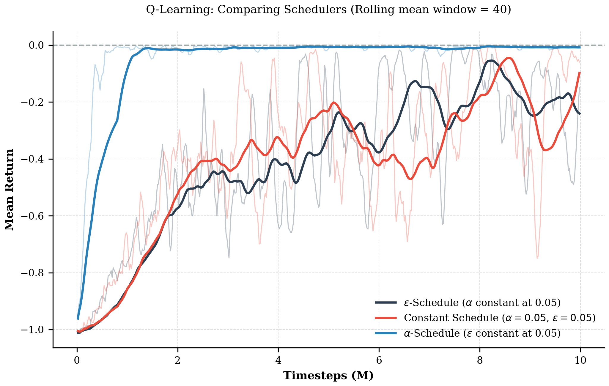
Q-learning returns did not improve monotonically because exploratory actions could still terminate an otherwise successful episode, while bootstrap targets continued to change as poorly visited parts of the large table were updated. A learning-rate schedule was especially important: it allowed large early updates and increasingly stable estimates later in training.
We used a state-action visit-count schedule for the learning rate, so rarely visited pairs received larger updates while frequently updated values gradually stabilized:
where $N_t(s,a)$ is the number of updates to $(s,a)$. We used $c=1.0$, $\omega=0.85$, $\gamma=0.99$, and $\alpha_{\min}=10^{-4}$. Exploration followed an inverse-decay schedule:
Here, $\epsilon_0=0.05$, $\epsilon_{\min}=0.01$, and $T_{\mathrm{total}}=10$ million steps. The $\alpha$-schedule controls how strongly the Q-values change, whereas the $\epsilon$-schedule controls which actions are sampled.
Figure 4. Q-learning behavior under different learning-rate and exploration schedules.
Using constant learning and exploration rates produced a final return of $-0.0852\pm0.2455$. The learning-rate scheduler improved this to $-0.00268\pm0.00227$, while combining the learning-rate and exploration schedules gave the strongest stability at $-0.00236\pm0.00193$.
Q-learning achieved the best average return, $-0.0018$, while MPC achieved a mean cost of $0.0060$ and DP achieved $0.0160$. MPC was slightly more consistent and had the better worst case; Q-learning occasionally encountered failures caused by discretization and insufficient coverage of less-visited states.
The methods also place computation in different locations. DP performs expensive sweeps over the complete $R^4$ grid, and Q-learning shifts the cost to millions of sequential interactions. Both produce policies that are inexpensive to execute. MPC instead solves an optimization problem online at every timestep, trading computation for immediate reactivity.
Changing the pole length exposed the limitation of a fixed learned policy. The Q-learning agent was trained at $L_0=0.5$ m, and performance degraded as evaluation moved away from this value because the transition dynamics changed. MPC is theoretically better suited to adaptation when its model can be updated, since it uses the latest state and model to re-plan online.
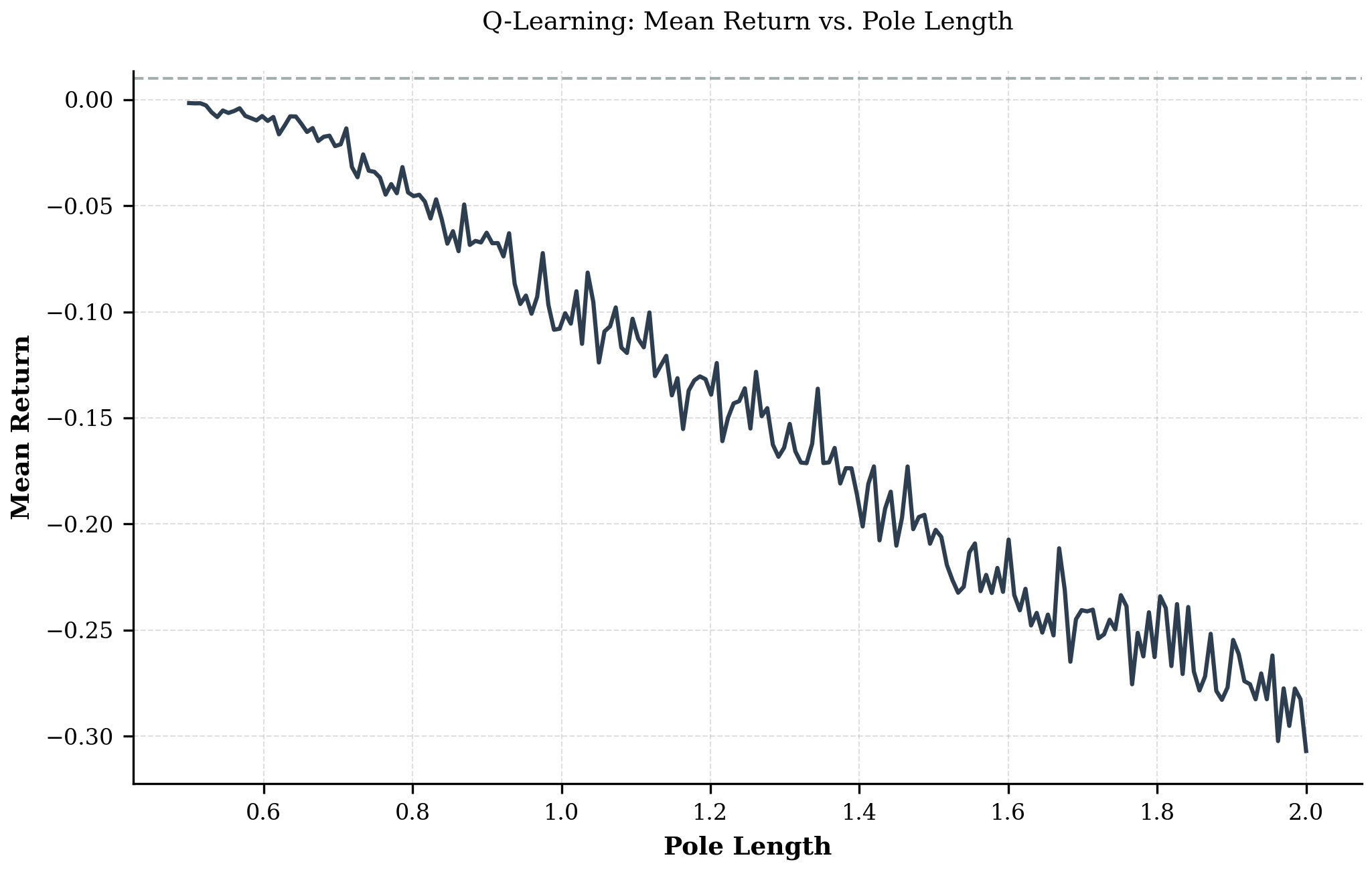
Figure 5. Q-learning return under pole-length perturbations after training at $L_0=0.5$ m.
No single approach dominated every criterion. DP offered interpretable grid-level optimality but suffered from the curse of dimensionality. Q-learning achieved strong average performance and inexpensive execution after substantial offline training, but was less reliable in rare states and under model mismatch. MPC required more online computation, yet its continuous re-planning made it the strongest basis for responding to disturbances and changes in the physical system.